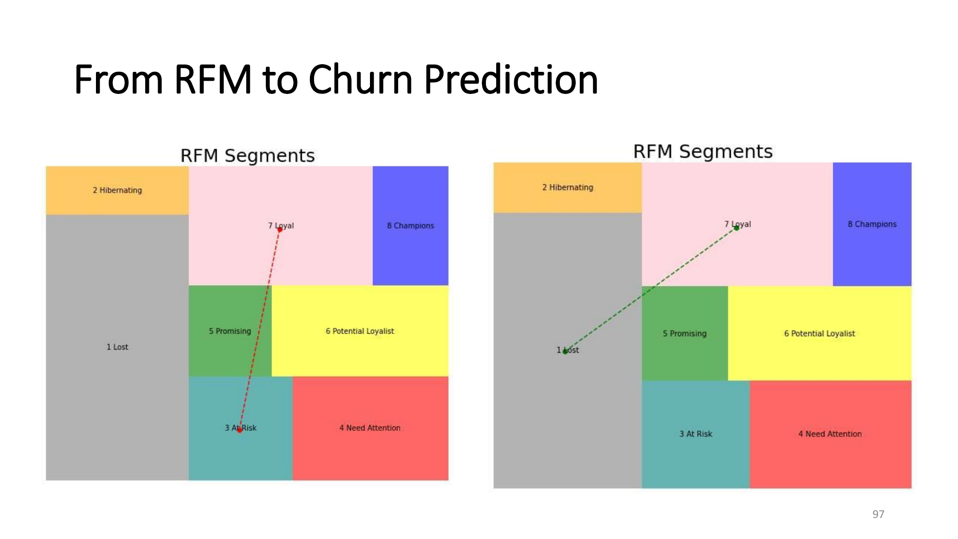
RFM is not only for segmentation. It reveals how a customer relationship moves.
Choose one customer and read three pieces of evidence together: how recently they returned, how often they purchased, and how much value they generated. Then inspect multi-period slopes to separate fading engagement from a naturally long repurchase cycle.
ONLINE RETAIL · REAL DATA · 541,909 SOURCE ROWS
Ready to experiment? Start here.
Every lab uses the same 18,532 valid invoices and population of 4,338 anonymized customers.
01 · DATA GRAIN
Before calculating, prove that the same customer can be followed over time.
The lab uses the real 541,909-row Online Retail dataset from 1 December 2010 to 9 December 2011—the same source used by the original SQL, notebooks and slides. Missing IDs, cancellations, negative quantities and zero prices are removed before product lines are aggregated into invoice rows.
Customer IDs are hashed into R-xxxxxxxx identifiers and the raw file remains outside the public web directory. Preparation yields 18,532 invoices from 4,338 customers, with a twelve-customer teaching cohort selected for contrasting behaviour.
COMMON DATA CONTRACTcustomer_id · invoice_id · occurred_at · amountOne row = one valid invoice after line aggregation; monetary values are GBP.
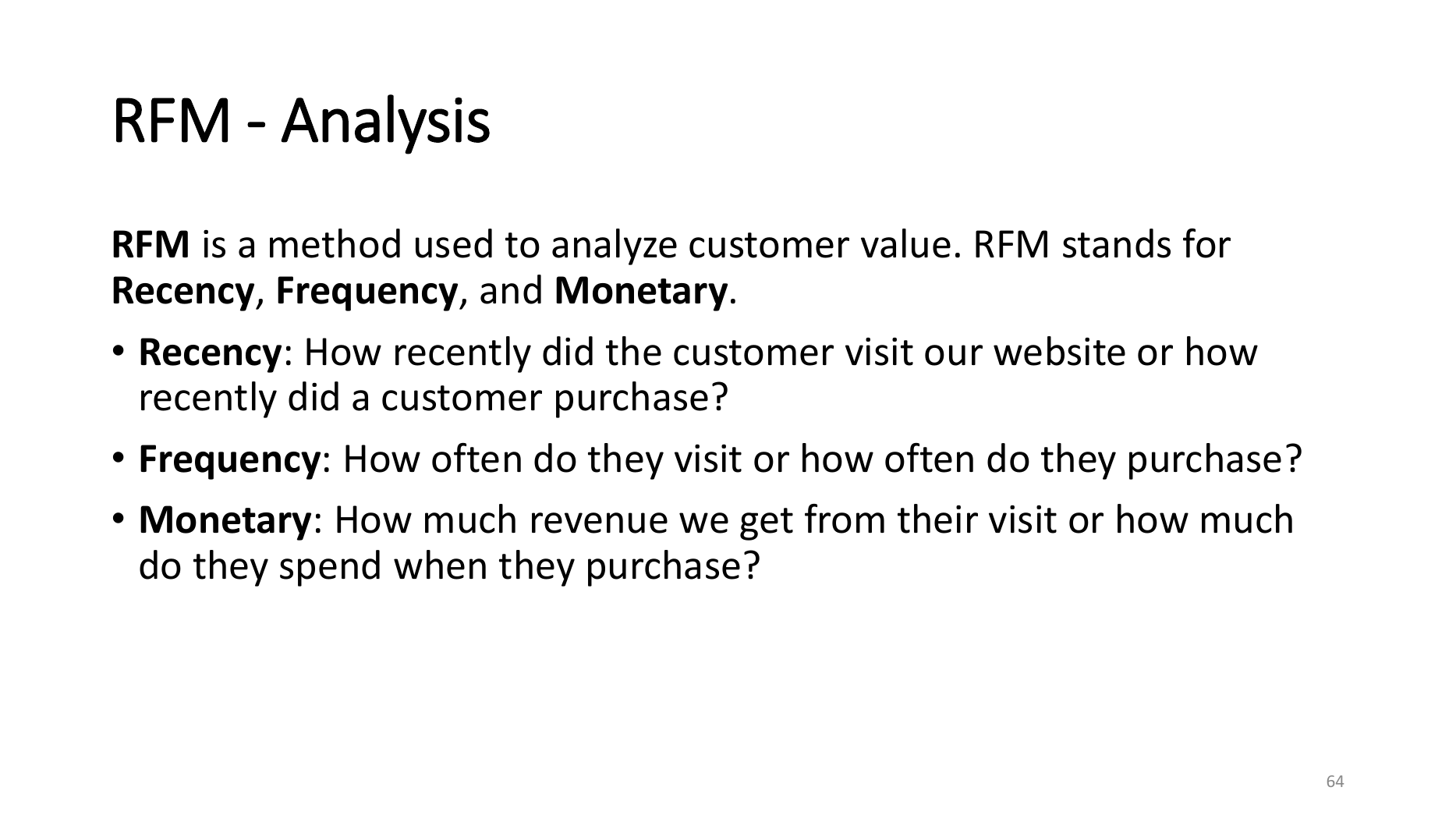
R · F · M ARE THREE DIFFERENT QUESTIONS
Do not combine the three too early. Each tells a different story.
RFM is attractive because its formulas are simple while its interpretation is not. We are not merely asking who spent the most; we measure distance, continuity and relationship size at a particular point in time.
R
Recency
How fresh is the relationship?
Count days from the last transaction to the snapshot. Lower is often better, but daily goods and annual purchases cannot share one threshold. Read recency against the expected purchase cycle.
R = snapshot_date − max(purchase_date)F
Frequency
Does the relationship repeat?
Count distinct invoices, not product rows; otherwise one basket with ten items appears as ten purchases. Define the window explicitly because lifetime frequency automatically favours older customers.
F = count(distinct invoice_id)M
Monetary
How much value arose in the same boundary?
Gross sales, net sales, margin and contribution are different. This lab uses paid amount for formula clarity; a real system should use the value aligned with the decision and handle refunds and cancellations correctly.
M = sum(valid transaction value)
BEFORE YOU RUN
Should the answer change when snapshot or window changes?
Predict the selected customer segment first.
Compare 90, 120 and 180-day windows.
Separate behavioural change from definition change.
R = snapshot − last purchaseF = distinct invoices in windowM = Σ invoice amount in window
RECENCY · lower is more recent—daysR—FREQUENCY · distinct invoices—ordersF—MONETARY · window value—THBM—RFM SEGMENT—RFM —
RAW METRIC ≠ RFM SCORE
Fourteen days does not always mean R = 4.
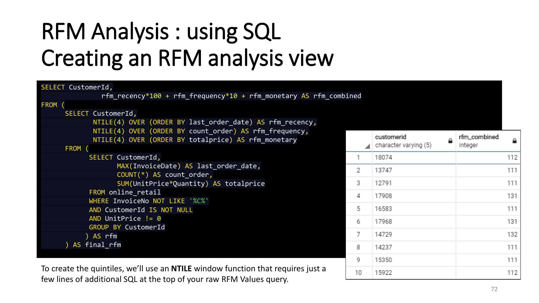
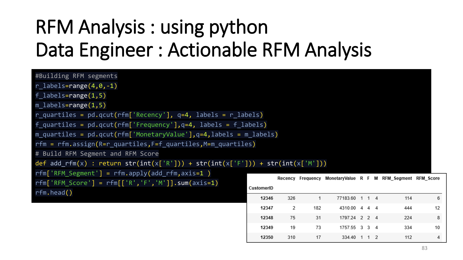
The raw metric describes the customer; a 1–4 score describes relative position within the population at the same snapshot. This lab uses quartiles: recency is reversed because lower is better, while frequency and monetary reward higher values.
When population or period changes, a score can change while the raw value stays constant. A feature store should retain raw values, binning logic and segmentation version.
04–05 · CUSTOMER MOVEMENT
Read the direction—not a single snapshot.
Each point uses the same rolling window; a line is fitted to values normalized within that customer.
Recency riskFrequencyMonetary
RECENCY SLOPE—
Positive means days since last purchase are rising—a negative signal.
FREQUENCY SLOPE—
Negative means rolling-window purchase frequency is falling.
MONETARY SLOPE—
Negative means rolling-window monetary value is falling.
CHURN SIGNAL · NOT A CALIBRATED PROBABILITY
—
—/ 100
HOW TO READ THREE SLOPES
Customers with the same falling score may require different responses.
R slopeF slopeM slopePossible readingInspect next
↑↓↓Broad disengagement
Product, channel, service issues and alternatives.
↑≈↑Less frequent, larger baskets
Possible order consolidation rather than churn.
≈≈↓Still returning, lower spend
Product mix, discounts, unit price and economic context.
↑↓≈Repurchase cycle may be lengthening
Compare category cadence and matched cohorts.
06 · FROM SIGNAL TO ACTION
A score should not make the decision. It should tell us what to inspect next.
Boundary to state clearly
The slope in this lab is a behavioural heuristic, not a trained and calibrated churn probability. A predictive model needs a churn horizon, future-derived labels, temporal validation, precision/recall and calibration checks, plus the product’s natural repurchase cycle.
FROM RFM HEURISTIC TO CHURN MODEL
To call it prediction, the future must provide the label.
RFM and slopes are useful, explainable features, but a model is credible only when every feature is built at prediction time without seeing the future.
01
Define the event
For example, no purchase within 60 days after snapshot, aligned with product cadence.
02
Build point-in-time features
Use RFM, slopes, tenure, interval variance, product diversity and refund rate from pre-snapshot data only.
03
Split by time
Train on the past, validate on the next period and test on the latest period; do not leak future rows through random splitting.
04
Evaluate for the decision
Use precision, recall, PR-AUC, lift@k and calibration alongside contact cost and retention value.
STUDENT INVESTIGATION
Questions students should answer after the lab
Why must frequency count distinct invoices, and what breaks when product rows are counted?
Does the same customer change segment under another window, and is that behavioural change or an artefact?
When can recency worsen without implying churn?
Why is a score of 80/100 here not an 80% churn probability?
Which labels and validation design turn a signal into a prediction?
FORMULA → SQL
Translate the same question into an inspectable query.
SELECT customer_id,
       DATEDIFF(:snapshot, MAX(occurred_at))                         AS recency,
       COUNT(DISTINCT invoice_id)                                   AS frequency,
       SUM(amount)                                                  AS monetary
FROM transactions
WHERE occurred_at > :snapshot - INTERVAL 120 DAY
  AND occurred_at <= :snapshot
GROUP BY customer_id;
In production, persist weekly or monthly snapshots and estimate slope by regression over multiple points rather than dividing two period scores once.
THE SAME RFM IDEA · TWO COMPUTATIONAL LANGUAGES
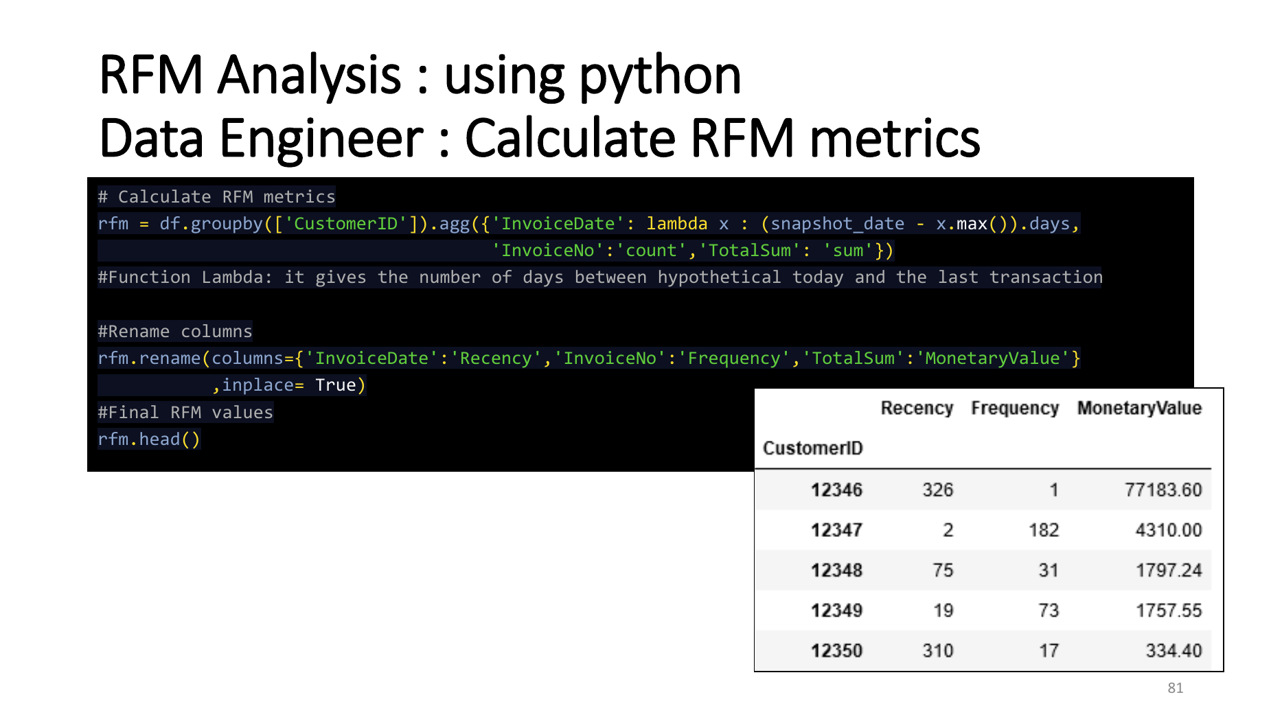
The notebook makes the process visible; SQL keeps it close to the data.
Read the question first, then translate the same formula between dataframe and relational operations in the slide sequence.
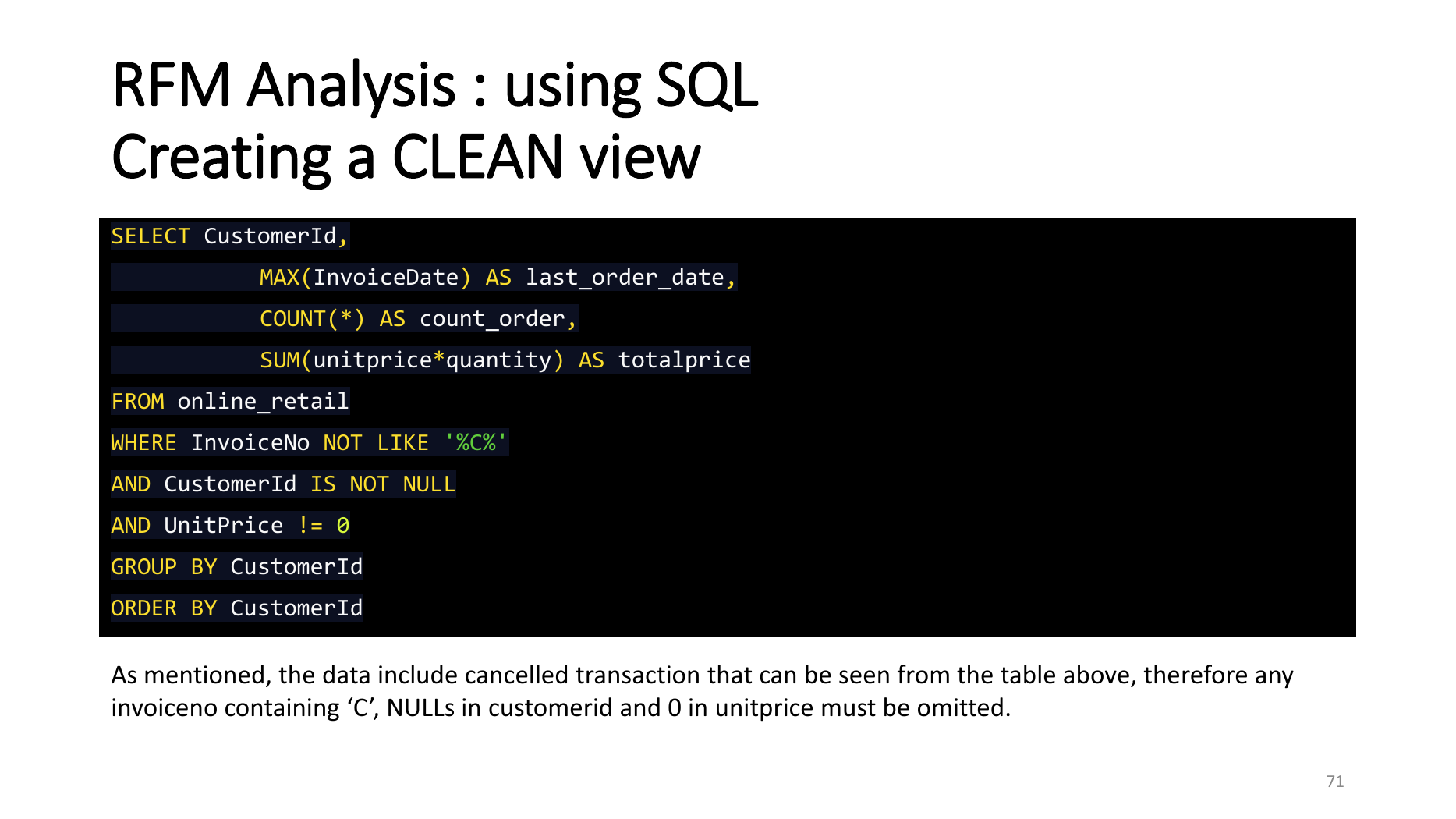
The original SQL uses COUNT(*) and directly ranks last_order_date. This lesson first counts distinct invoices and derives elapsed days from a snapshot so Frequency and Recency match their definitions.
FROM THE ORIGINAL LECTURE · VISUAL READING
The original slides show how RFM moves from tables to segments and movement.
These are not a decorative gallery. They follow the reasoning sequence: definition → query → metrics → scoring → visualisation → churn signal.
01 · DEFINEBegin with three distinct questions before combining them into one score.
02 · CLEAN VIEWSQL aggregates transactions by customer and defines valid data boundaries.03 · SCORE IN SQLWindow functions translate raw metrics into relative population positions.
04 · CALCULATEThe notebook exposes snapshot logic, aggregation and the result table together.05 · SCORE IN PYTHONqcut forms quartiles and combines R, F and M into an interpretable code.
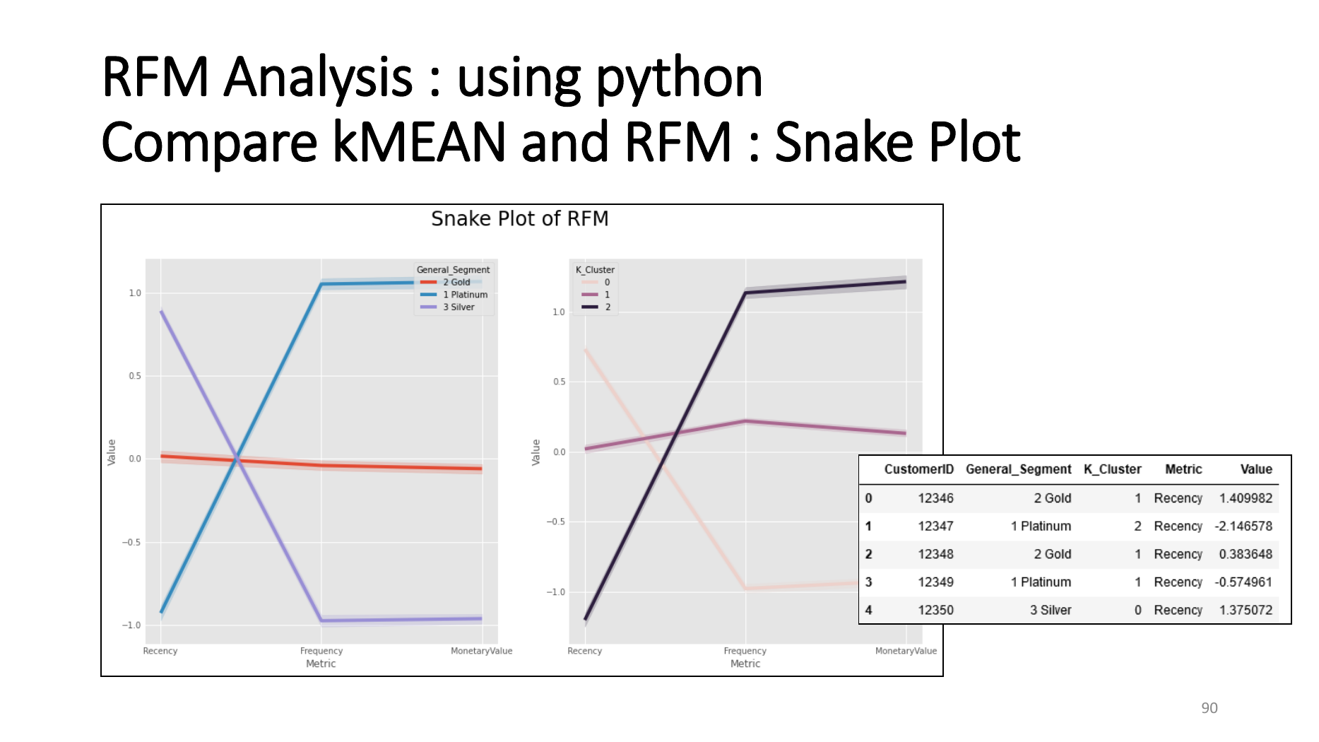
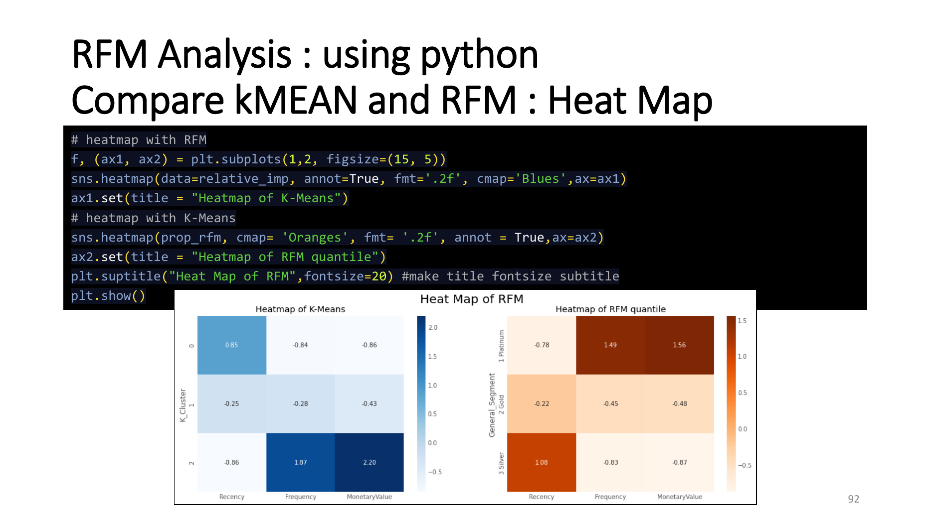
06 · READ SHAPEA snake plot reveals which metric distinguishes each group—not merely the total score.07 · COMPARE PROFILESHeat maps expose relative RFM importance across segments.
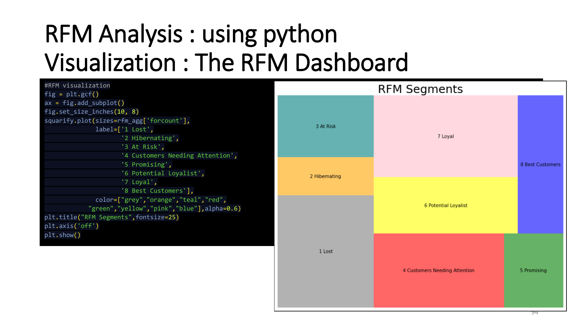
08 · SEGMENT MAPSegment area conveys population size; position and labels support business communication.09 · MOVEMENTMovement between segments bridges segmentation and churn signals, but is not yet a probability.
Teaching prompt
SQL and Python agree when data contract, snapshot, filters and quartile logic agree. If results differ, first inspect grain, cancelled invoices, distinct-invoice counting, ties and snapshot boundaries—not the engine.
BOUNDED PYTHON RUNNER · LIVE DASHBOARD
Choose a stage and run the real Python calculation.
This dashboard exposes parameters, not arbitrary execution. The displayed code is the actual bounded operation, allowing students to read, run and inspect output without opening a server shell.
CONNECTING…— ms
PYTHON CODE · READ ONLY
# Select an operation and run.
RESULT · JSON
{}
Safety boundary
Only four operations, twelve customer IDs and bounded snapshots/windows are accepted. There is no eval/exec, package installation, user filesystem access or public Python-service port.
ROLLING TIME WINDOW · DYNAMIC RFM
As time moves, RFM can change even without a new row.
Move the snapshot or press Play and watch both boundaries: the right edge is “today,” which increases recency; the left edge expires evidence, reducing frequency and monetary value when transactions fall out.
——
Expired
ROLLING WINDOW
Future
+ 0 entered− 0 expired0 inside
RECENCY—days since last purchase—FREQUENCY—invoices in window—MONETARY—THB in window—
Recency riskFrequencyMonetary
01 · No new purchase
Recency rises with time; F and M hold until the left boundary reaches a transaction.
02 · A new purchase arrives
Recency resets near zero, frequency increases and monetary value rises by the transaction amount.
03 · An old purchase expires
Nothing is deleted from the database; the feature changes because the window no longer sees that evidence.
RFM SEGMENT MAP · CUSTOMER MOVEMENT
Where is the selected customer—and where are they moving?
The map scores all 4,338 customers for the selected snapshot and window. The dashed outline marks the previous position; the solid outline marks the current one.
LOADING POPULATION…4,338 customers scored
Read with care
A segment is a business rule translating RFM scores into shared language, not a permanent truth. Changing the snapshot, window, or population quartile boundaries may move a customer.